We will use python bundled with a few key scientific libraries (Numpy, Scipy, and Matplotlib) in an installation called "Anaconda" that you can download from here. To determine whether your system has a 32-bit or 64-bit processor, see the following links: Mac Users or Windows Users.

Part II: Getting Started and Recording Your Work

After installing Anaconda, find the "Spyder" app in the installation folder or your programs menu, which will provide a nice user interface. Spyder may take a while to start up, because of all the python libraries it is loading.


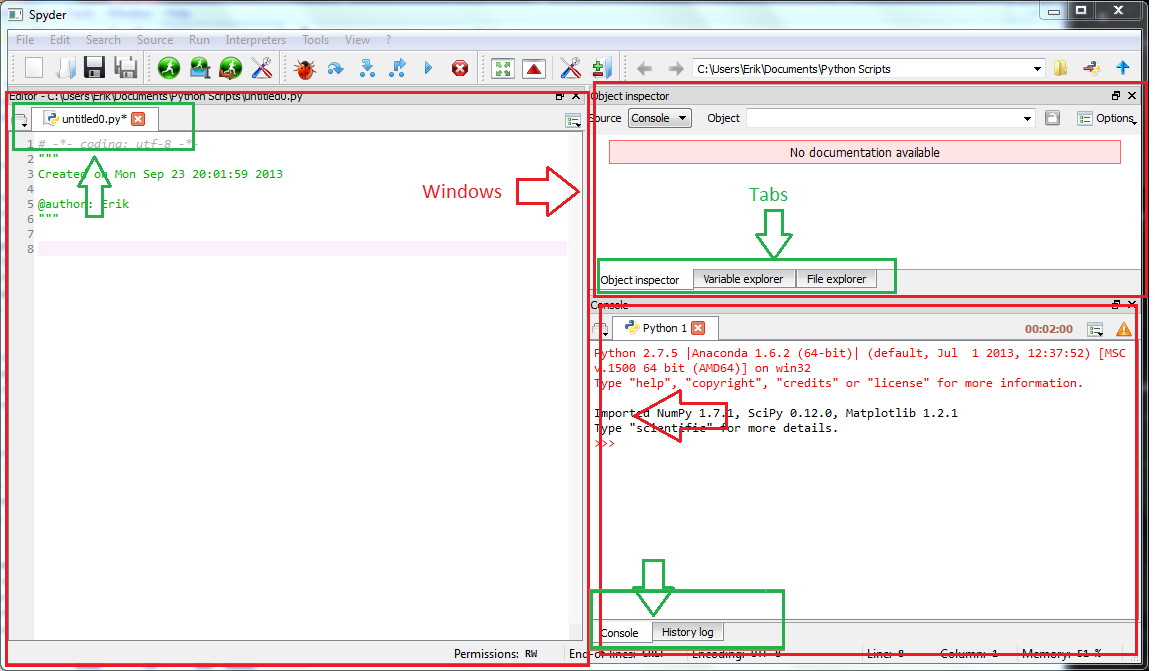
The first thing to note is how the Spyder app is organized. The application includes multiple separate windows (marked with red rectangles), each of which has its own tabs (marked with green rectangles). You can change which windows you prefer to have open from the View -> Windows and Toolbars option. The default configuration has the Editor, Object inspector/Variable explorer/File explorer, and Console/History log windows open as shown above (except that the Variable explorer tab is missing in the screenshot).

The Console is where python is waiting for you to type commands, which tell it to load data, do math, plot data, etc. After every command, which looks like >>> command, you need to hit the enter key (return key), and then python may or may not give some output. The Editor allows you to write sequences of commands, which together make up a program. The History Log stores the last 100 commands you've typed into the Console. The Object inspector/Variable explorer/File explorer windows are purely informational -- if you watch what the first two display as we go through the tutorial, you'll see that they can be quite helpful.

Entering Data
Type "x=5" in the Console -- this is the command to create a variable named x and give it the value 5. If you raise the "Variable explorer" tab you will see that x has been added to the list of variables in python's memory. You can also type "print x" or even just "x" in the Console to see the value of x. Now type "y=4" and then "x+y". Notice that this last command does not create a variable, although it does produce an output from the calculation.

Arrow Keys
If you use the arrow keys in the Console, you can bring back a previous command so that you can edit and re-execute it. Go back to the command "x+y" and change it to "junk=x+y". You've now created the variable junk. What can you type to see its value in the Console?

Arrays
Python can work with arrays of numbers, such as columns of data or tables of data (rows and columns). However, by default it is set up to handle lists of any kind of data -- perhaps names or addresses, not just numbers -- so we have to use the "array" function from Numpy (numerical python) to tell python that a given set of numbers should be treated as a numerical array. Before we do this, we need to learn the syntax for calling functions from a library.

Interlude on Libraries Behind the scenes, Anaconda installs the libraries Numpy, Scipy, and Matplotlib to give you access to thousands of special functions. Every time you want to call one of these functions, you must first type the name of the library, followed by the name of the function like so "Library.Function". Furthermore, the library must have been "imported" before you type this command. The Console automatically imports Numpy, Scipy, and Matplotlib at startup, as well as the sublibrary "pyplot" from Matplotlib, and it also gives the libraries nicknames so you don't have to type the whole name out (np, sp, mpl, and plt respectively). However, you would need to do this manually in any program you wrote in the Editor window, for example by starting the program with the command "import Numpy as np". Type "scientific" into the Console to see the full list of commands executed by the Console on startup.

Interlude on Comments The # signs after each command output by "scientific" indicate comments explaining what these commands do. Comments are ignored by python and not executed. They are very useful for reminding yourself what a program is actually doing when you go back to look at it a few months after writing it.

Now back to arrays. We wish to create a numerical array, as opposed to a list of numbers. To see how these differ, first type

>>> x=np.array([1,2,3,4])
>>> y=np.array([4,0,3,2])
>>> z=x+y
>>> print z

and look at how these variables appear in the Variable explorer. Now type

>>> x=[1,2,3,4]
>>> y=[4,0,3,2]
>>> z=x+y
>>> print z

and compare. For present purposes, we are not interested in the "list" behavior of the second set of commands, but only the "array" behavior of the first set. It's also worth noting that python happily overwrites x, y, and z with no error message, even when it means changing their variable types -- this behavior is different from that of programming languages that declare variables.

When working with real data, we may have both rows and columns. For example, define "x=np.array([[1, 3] , [2, 4], [10, 11]])". The brackets within brackets imply 3 rows and 2 columns.

If you want to pick out one or more rows/columns in the array, you must use "indices" (a.k.a. "subscripts") to identify the portion of the array you want -- rows first, columns second, in square brackets. Both are numbered starting from zero. The colon ":" indicates a range, with two odd features -- first, "x:y" actually means index numbers from x to (y-1), and second, ":" by itself means all index numbers. For example, compare the results of "out1=x[1:2,1:2]" with the result of "out2=x[0,:]". In the first example the colon acts like a dash specifying a range, i.e., read "1:2" as "1 to (2-1)" which is "1 to 1" or just the single index 1. The first command says you want out1 to be restricted to row #1 (the second row) and column #1 (the second column) of "x", while the second says you want out2 to equal row 0 (the first row) of "x" with all columns. We refer to each number in an array as an element. Try to write a command to select the element of "x" in the second row, first column, and assign it to "y".

Special Arrays
Numpy's "arange" function can be used to generate a series of numbers, either in +1 increments (the default) or in increments you specify. Compare the output of "x1=np.arange(1,5)" and "x2=np.arange(1,5,2)". The final number is the increment, unless it's missing, in which case it's assumed to be 1. The first two numbers are the starting and ending points, but once again python stops one increment before the ending point, just as for subscript ranges.

The "zeros" command can also be useful to make arrays you want to fill in with nonzero values later. For example, type "newarray=np.zeros([4,3])" and "x1=np.arange(1,5)". Examine these variables dimensions under the "Size" column in the Variable explorer, or type "newarray.shape" and "x1.shape" to output their dimensions. Now type "newarray[:,1]=x1". Examine the result carefully -- why was it necessary to use subscripts on newarray before inserting x1? Try "z=newarray+x1". It gives an error -- why?

Simple Math
Although python can do advanced math, we won't need that, so you should just remember a few simple operators and functions:
+ addition
- subtraction
* multiplication
/ division
** to-the-power-of
e times 10-to-the (e.g. 2.e4 = 2 .* 10^4)
abs() absolute value
sqrt() square root
exp() e^
log() natural log or ln
log10() ordinary log (opposite of 10^)
sin() sine of angle in radians
cos() cosine of angle in radians

Note that the operators listed above do math "element-wise", meaning if you, e.g., multiply two single column arrays, the two first elements will multiply, the two second elements will multiply, the two third elements will multiply, etc. Unlike matlab, python does not treat "*" as matrix multiplication for arrays, rather as simple element-wise multiplication.

Now using parentheses and simple math, you can create your own functions. For example, suppose you'd like to define a column of data (one-dimensional array) that obeys the equation c=lambda*nu over a range of lambda from 300-700nm going up by 50nm at a time. You can type "lam=300.+np.arange(0,401,50)" first, then "nu=3.e17 / lam" (where the speed of light is 3 x 10^17 in units of nm/sec). The output should be nu in Hertz (1/sec). Notice that although the "300." was a scalar, python allows you to add it to an array (all elements) and does not complain about size mismatch. Warning: don't try to use the variable name "lambda" instead of "lam"! The word "lambda" has a special meaning in the python programming language, which we don't need to get into.

Use parentheses liberally! It is very easy to do different math than you intend. Notice that "nu=3.e17 / 300.+np.arange(0,401,50)" does not work properly, although you could write "nu=3.e17 / (300.+np.arange(0,401,50))".

Multi-Element Math
You might like to compute some overall properties of a data set. We'll save some tricks of this type for later, but try these simple ones: sum, max, min, median, mean. You can see how these functions work by creating a 3x3 array of random numbers (for this you will need a special sublibrary of Numpy called "random", so the syntax is "x=np.random.rand(3,3)") and then computing each statistic, e.g., "mean(x)".

What else is out there?
Extensive lists of additional functions available to you can be found here: Numpy, Scipy, and Matplotlib. Moreover, there are dozens of other python libraries we will not be using -- someday you may create your own library!

Logging Your Work
Now that you've seen the basics, let's start recording your work. To do this, you should paste all your successful commands from the History or Console window into the Editor window, where they will become a program (sequence of commands). Do NOT paste in the ">>>" from the Console, but please DO paste in the output from your successful commands, inserting a "#" comment character before each line of output so that python does not try to interpret the output as a command. The program file in the Editor window will initially be labeled ".temp.py" but you should save it under the new name "tutorialanswers_yournamehere.py" in a different folder that you will use for all your python files. Also put a comment at the top with your name and date, and make sure to explicitly insert the startup file commands we saw when we typed "scientific". Now you can check your answers by saving and running your program with the "save" (disk icon) and "play" (green arrow icon) buttons at the top of Spyder. You will submit your final program file as part of your homework.

At last, it's time to show off your new python skills "for the record."

(1) Using "arange", create an array called "myarray" that has the same length as the number of letters in your last name and counts up from 1.
(2) Create a second array that is the square root of the first. Call the second array "rootarray". How many elements are in "rootarray"? If it's not the same as the number of letters in your last name, you have a problem.
(3) Compute myarray divided by rootarray. You can name the result "ratio". Careful! Check that myarray has more than one element. If it doesn't have the same number of elements as the number of letters in your last name, go back and review the section on "Simple Math" above.
(4) Multiply ratio times rootarray. Does the result make sense?
(5) Add a comment to your program file to answer the question from (4), i.e. explain why the result makes sense.

The final version of your program file should contain only successful commands and their output -- please leave only your most brilliant work for the grader.

Part III: Reading and Plotting Data

First, download testdata.in into the directory where you keep your python files -- this should be the same one where you put "tutorialanswers_yournamehere.py" earlier. Reading the data is now simple: just type

data=np.loadtxt(r"XXXXtestdata.in")

where "XXXX" should be replaced with the path to your file (displayed at the top of the Editor Window if you put your program and data files in the same place as instructed). An example might be "C:\My Documents\Python Scripts\". The extra "r" in front of the path and filename is necessary to force python to interpret the information literally. Note that loadtxt *assumes* your data is in numeric form, so if there's a header with column names, you should remove that before reading.

Now, you have all your data in one array. If you want to work with different columns, it is helpful to name them and extract them from the array. For example:
temperature=data[:,0]
humidity=data[:,1]

To plot temperature vs. humidity, you can just type "plt.plot(humidity,temperature)" where the desired x-axis is listed first. This should pop up a plotting window with the data points connected by lines -- rather a mess.

To beautify this plot, we can specify the output more: "plt.plot(humidity,temperature,'b.',markersize=12)" will use blue dots with dot size 12 (most obvious colors work, e.g. r for red, g for green -- see summary here). Type this in, then look back at the plot window. Unfortunately, the mess is still there, we just overplotted points on top of it. Type "plt.clf()" to clear the figure, then try the same thing again: "plt.plot(humidity,temperature,'b.',markersize=12)". This should look much better.

Now, to add axis labels and a title, type the following:

plt.title('Fantastic Plot #1')
plt.xlabel('humidity (%)')
plt.ylabel('temperature (F)')

You can also change the axis ranges, like so;

plt.xlim(10,60)
plt.ylim(75,100)

Alternatively, these options can be set interactively from the plot window if you click on the check mark at the top. You can also click on the four-way arrow and drag your right mouse button inside the plot to resize the axes. For example, try using these plot window capabilities to zoom in on the humidity range from 10-40 and the temperature range from 80-100, thus excluding the two outlying data points in the plot. Of course, scientific integrity demands that you should never cut out a "bad" data point from a real data set without explaining why you're doing so, and having a very good reason!

Suppose you wanted to subselect certain data from your dataset for a legitimate reason, for example, let's say you just want to look at the temperature on days with humidity less than 20%. Rather than looking through the data, you can use the Numpy "where" function to select out those particular days. Type in "sel=np.where(humidity < 20)" and "print sel", so that you can see what sel is. What are the numbers in sel? Inspection in the Variable explorer shows that these numbers are the indices of the data points that meet our criteria (humidity is less than 20%). To check that sel does indeed find the data points where the humidity is less than 20%, type "print humidity[sel]". Now come up with a command to show the temperature values where the humidity level is < 20%. To check your answer, the temperature values should be: 89 and 93.

You can join multiple selection criteria together by using the "&" sign. Let's say rather than zooming in on your plot like we did earlier, you decide you just want to plot the data that meet certain criteria, i.e., temperature ranges from 80-100 and humidity from 10-40. To start this selection, write "sel2=np.where((temperature > 80) & (temperature < 100))". Go ahead and overplot this selection: "plot(humidity[sel2],temperature[sel2],'g*',markersize=15)". You should find that the overplotted symbols range from 80-100 in temperature. Finish the selection to restrict the humidity range from 10-40. Overplot using 'r+' (red plus signs). Put this final combined selection into your Editor file.

To finalize your plot so you can submit it with your program file, first retitle the plot with your name and the assignment, e.g., "Jane Doe Python Tutorial", then save it (the zoomed in version with the bottom right point cut out and red plus signs overplotted) to a file. If you save to pdf it should be easy to print. Print your program out from the Editor window as well (you can do this directly from Spyder) and hand it in together with your plot.